Showing posts with label BackToWorkMonday. Show all posts

Monday, December 11, 2023

Master the Magic of Excel: Unleash the Power of the Fill Handle

Microsoft Excel
Have you ever found yourself in a sea of data, manually copying formulas down a column in Excel? 

Have you ever wondered if there’s a faster, more efficient way? 

Here's a Cool Tip.  Use Microsoft Excel's most underutilized feature: the Fill Handle.

In Microsoft Excel, double-clicking the fill handle will automatically copy a formula down to the end of the data. 

The fill handle is a small black square in the bottom right corner of the active cell. 

When the pointer changes to a small black plus sign, you can double-click the fill handle to activate the AutoFill feature. 

www.OneCoolTip.com - Back To Work Monday

Here's how to do it.
  • Select the cell you want to copy.
  • Hover over the fill handle in the bottom right corner of the cell.
  • Double-click the fill handle.
  • The cells below will auto-populate based on the prior column and where you left off.
  • Scroll down to the bottom of your data to check if the formula has been copied correctly.

The Fill Handle can save you a significant amount of time, especially when dealing with large datasets. 

However, it’s important to note that it copies the exact formula, including relative cell references. 

If your formula includes absolute cell references, you may need to adjust them accordingly.


Excel Double Click Handle to Autopopulate

fig. 1 - Microsoft Excel - Double Click Selection Handle to Auto-Populate to End of Data


The Fill Handle is enabled by default in Excel. 

If it’s not working, check your settings: File > Options > Advanced > Enable fill handle and cell drag-and-drop.

Microsoft Excel - Enable Fill Handle
fig. 2 - Microsoft Excel - Enable Fill Handle


Please LIKE and SHARE OneCoolTip.com!
Visit the OneCoolTip YouTube Channelhttps://www.youtube.com/@onecooltip


READ MORE

OneCoolTip.com
Cool Tech Tips for a Cooler Life


#Microsoft @Microsoft #Excel #ExcelTips #DataAnalysis #ProductivityHacks #TechTips #OneCoolTip @OneCoolTip #YouTube 

Monday, December 4, 2023

How to Unlock Age Calculation in Excel

Have you ever wondered how to calculate someone’s age in Excel? 

Or have you tried to do it but found it more complicated than you expected? 

Here's a Cool Tip.  Use the DATEDIF in your formula, 

DATEFIF a hidden gem in Excel that makes age calculation a breeze.

www.OneCoolTip.com Back to Work Monday

Here's how to do it.
  • Open your Excel spreadsheet where you have the names and birthdates.
  • Insert a new column for ‘Age’.
  • Click on the first cell under the ‘Age’ column.
  • Type the DATEDIF formula: =DATEDIF(B2,TODAY(),"Y")
    • B2 should be the cell containing the birthdate
    • "Y" calculates the difference in complete years.
  • Press Enter and the age will be calculated.
  • Drag the fill handle (small square at the bottom-right of the cell) down to copy this formula to the rest of the cells in the ‘Age’ column.

Calculate Age in Excel with DATEDIF

fig. 1 - Calculate Age in Excel with DATEDIF


DATEDIF is a simple and easy to use once you understand how it works.

And it automatically updates the age as time progresses.

Enjoy!

Note:  Microsoft provides this functionality to support older versions of Excel.  It's possible that they will stop supporting it.


Please LIKE and SHARE OneCoolTip.com!
Visit the OneCoolTip YouTube Channelhttps://www.youtube.com/@onecooltip


READ MORE


OneCoolTip.com
Cool Tech Tips for a Cooler Life

#Microsoft @Microsoft #ExcelTips #DATEDIFFormula #AgeCalculation #ExcelTutorial #BackToWorkMonday #TechTips #OneCoolTip @OneCoolTip 

Monday, November 27, 2023

How to Master Microsoft Outlook Search

Have you ever found yourself sifting through hundreds of emails in your Microsoft Outlook inbox, trying to find that one important message? 

Ever wished there was a quicker way to locate specific emails?

Here's a Cool Back-to-Work-Monday Tip.  Use Microsoft Outlook Search Operators.

Here's how to do it.
  • Open Microsoft Outlook.
  • Navigate to the Search Box, located at the top of the Outlook window.
  • Type in the specific search operator you wish to use. 
    • For example, from:(sender) will show all emails from a specific sender.
  • Press Enter to display all emails that match your search operator.

But wait...  

There's a even Cooler Cool Tip.  Use the Outlook Search Filter screen.
  • Press and Hold the Filter icon to display search screen.

Outlook Search Screen
fig. 1 - Outlook Search Screen

  • Use the screen to enter your search criteria in one or more fields.
  • Then press Search to see the results.
But if you want to enter your own search operators, there are a number of operators that you can manually enter in the main search box.

Enter your search criteria in the Search box at the top of screen.


fig. 2 - Outlook Search

Using search operators can drastically reduce the time spent looking for specific emails, making your work more efficient.

Here are a few examples of search operators you can use:

from:(sender): 
Shows all emails from a specific sender.

subject:(keyword): 
Shows all emails with a specific keyword in the subject line.

NOT operator: 
This operator is used to exclude emails that contain a certain word.

OR operator: 
This operator is used to include emails that contain any of the specified words.

[ ] operator: 
This operator is used to search for empty fields.

to:
This operator searches the To line for emails addressed to a specified recipient.

cc:
This operator searches the Cc line for specified email recipients.

before:
This operator searches for emails sent or received before the given date.

after:: 
This operator searches for mail sent or received after the given date.

date:: 
This operator searches for mail sent or received on the given date.

folder:
This operator searches for mail in the specified folder.

has:attachment:
This operator searches mail messages that have at least one file attachment.

Remember, by default, you will be searching with the AND operator which you do not have to specify in your search. 

You can use the OR operator if you want your search results to also include items for which only a single condition is met. 

You can combine this field with the NOT operator to find items for which any value is selected.

For a full list of search operators, check out this Microsoft Support page.

That's it.

Enjoy!

Please LIKE and SHARE OneCoolTip.com!
Visit the OneCoolTip YouTube Channelhttps://www.youtube.com/@onecooltip


READ MORE


OneCoolTip.com
Cool Tech Tips for a Cooler Life

#Microsoft  @Microsoft #Outlook #Search #OutlookTips #EmailManagement #ProductivityHacks #TechTips #BacktoWorkMonday #OneCoolTip @OneCoolTip

Monday, November 13, 2023

How to Use Microsoft Excel's Geography Data Type Feature

Have you ever wondered how to make your Excel spreadsheets more dynamic and informative? 

Here's a Cool Tip.  Use Microsoft Excel's Geography Data Type feature.

Microsoft Excel’s geography data type feature is a powerful tool that allows you to access and integrate rich geographical data into your spreadsheets. 

But how does it work, and what can you do with it? 

Here's how to use it.
  • Start by typing geographic data into your cells. 
    • This could be country names, city names, or even postal codes.
  • Highlight the cells containing your geographic data.
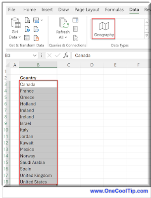
  • Navigate to the Data tab and select 'Geography’. 
    • Excel will automatically convert your data to the geography data type.
Microsoft Excel - Select Country Cells and Geography

fig. 1 - Select Country Cells and Geography

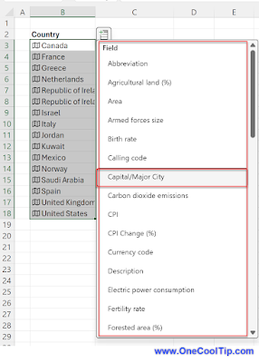
  • Click on the Insert Data button that appears when you select a cell with the geography data type. 
  • From here, you can choose what information you want to display in your spreadsheet.
Select Country Fields

fig. 2 - Select Fields

  • The geography data type feature in Excel offers  allows you to access a wealth of information about geographic locations.
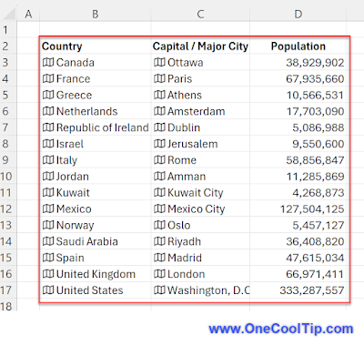
  • After converting them to the geography data type, you can extract information such as capital and  population, and more. 
Excel Geography Fields

fig. 3 - Excel Geography Fields

This can be incredibly useful for a variety of applications, from creating informative tables to performing data analysis.

The information in Excel’s geography data type feature is linked to an online data source, which means it can be refreshed and updated. 

To get current data for your data types, you can right-click a cell with the linked data type and select Data Type > Refresh or Refresh All

This will refresh the cell you selected, plus any other cells that have that same data type. 

This ensures that your data is always up-to-date with the latest information from the online data source.

Excel also has Stocks and Currency data types which we'll cover in a future Cool Tip.

Enjoy!

Watch this Cool Tip video to learn more about using Microsoft Excel's Geography Data Type feature:


Please LIKE and SHARE OneCoolTip.com!
Visit the OneCoolTip YouTube Channelhttps://www.youtube.com/@onecooltip


READ MORE

OneCoolTip.com
Cool Tech Tips for a Cooler Life


#Microsoft @Microsoft #Excel #MicrosoftExcel #ExcelTips #DataScience #MicrosoftOffice #TechTips #BackToWorkMonday #YouTube @YouTube #OneCoolTip @OneCoolTip 

Monday, November 6, 2023

Boost Your Productivity with Microsoft Excel's Paste as Picture

Microsoft Excel
Have you ever wondered how to make your Excel reports more visually appealing? 

Or how to keep your data updated across multiple sheets without the hassle of manual updates?

Here's a Back-to-Work-Monday Cool Tip.  Use Microsoft Excel's Paste as Picture.

Microsoft Excel, a powerful tool in the Microsoft Office suite, offers two unique features: Paste as Picture and Paste as Linked Picture

While they may sound similar, they serve different purposes and can be used to achieve different outcomes.

Here's how to do it.

Paste as Picture
This feature allows you to take a snapshot of your selected cells and paste it as an image. 
  • Select the cells you want to copy.
Microsoft Excel - Select Table to Copy

fig. 1 - Select Table to Copy

  • Go to the Home tab, click on the Copy dropdown, and select Copy as Picture.
  • In the dialog box, choose “As shown on screen” and “Picture”, then click OK.
Microsoft Excel Copy as Picture
fig. 2 - Microsoft Excel Copy as Picture
  • Go to the location where you want to paste the picture and press Ctrl+V.

It’s a great way to preserve the look of your data, especially when sharing it with others.

The pasted picture won’t change even if the original data is modified.

Paste as Linked Picture
This feature creates a live snapshot of a range of cells. 
  • Select the cells you want to copy.
  • Copy the cells (Ctrl+C).
  • Go to the Home tab, click on the Paste dropdown, and select Linked Picture.

Microsoft Excel - Paste as Linked Picture

fig. 3 - Microsoft Excel - Paste as Linked Picture

The linked picture updates automatically when the original data changes.

It’s useful for creating dynamic dashboards and reports.

Here’s an example to illustrate the difference. 
  • Let’s say you have a cell A1 with the value 10. 
  • If you use Paste as Picture, you’ll get a picture of the cell displaying 10. 
  • If you change the value in A1 to 20, the picture remains the same. 
  • But if you use Paste as Linked Picture, the picture will update to display 20.
Be sure to check out this video that explains Paste as Picture and Paste as Linked Picture.


Enjoy!

Please LIKE and SHARE OneCoolTip.com!
Visit the OneCoolTip YouTube Channelhttps://www.youtube.com/@onecooltip

READ MORE

OneCoolTip.com
Cool Tech Tips for a Cooler Life

#Microsoft @Microsoft #Excel @Excel #ExcelTips, #DataVisualization, #ProductivityHacks, #MicrosoftExcel #TechTips #YouTube @YouTube @OneCoolTip @OneCoolTip 

Monday, October 30, 2023

How to Quickly Create a Table in Microsoft Word

Have you ever wondered how to create a table quickly in Microsoft Word ?

Maybe there's a quick keyboard shortcut?

How about an "old school" trick?

Here's a Cool Tip.  Use simple ASCII characters.

Here's how to do it.
  1. Open Microsoft Word. 
  2. Type a plus sign (+) followed by a series of minus signs (-) and end with another plus sign (+). 
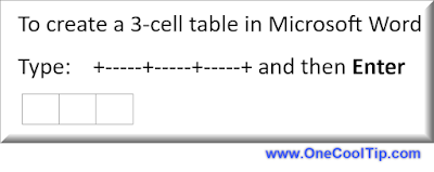
  3. For example, to create a 3 cell table, type: +-----+-----+-----+ and then Enter.

Create a Table in Microsoft Word

fig. 1 Create a Table in Microsoft Word Using + and -s


    4. Just follow the pattern to create a table with more columns.
    5. Click into the last cell and press Tab key to create a new row.

Creating tables with ASCII characters is quick and easy. 

It’s also a fun way to impress your colleagues with your Word prowess!

Enjoy!

Please LIKE and SHARE OneCoolTip.com!
Visit the OneCoolTip YouTube Channelhttps://www.youtube.com/@onecooltip

READ MORE


OneCoolTip.com
Cool Tech Tips for a Cooler Life


#Microsoft @Microsoft #Word #MicrosoftWord #WordTips #ASCII #Productivity #TechTips #OneCoolTip @OneCoolTip 

Monday, October 23, 2023

Unleash the Power of Online Videos in Microsoft Word

Microsoft Word
Have you ever wanted to make your Microsoft Word documents more engaging and interactive? 

Are you tired of sending just links to videos in your documents? 

Here's a Back-To-Work-Monday Cool Tip.  Use the Insert Online Videos feature in Microsoft Word.

Insert Online Videos is a feature in Microsoft Word that allows you to embed videos from online sources, such as YouTube, Vimeo, and SlideShare.net, into your Word documents. 

This can be a great way to add multimedia content to your documents, such as instructional videos, product demos, or engaging presentations.

Here's how to do it.

Insert Online Videos in a Microsoft Word document.
  1. Open your web browser.
  2. Navigate to the video you want to embed
  3. Microsoft Word supports inserting videos from a number of sites including Vimeo, YouTube, and SlideShare.net.
  4. Copy the URL.
  5. Open the Word document where you want to insert the video.
  6. Click on the Insert tab in the ribbon.
  7. Click on Online Videos in the Media group.

Insert Online Video in Microsoft Word
fig. 1 - Insert Online Video in Microsoft Word

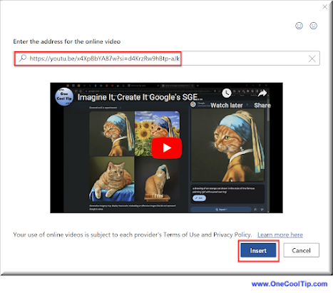
  1. In the Insert Video dialog box, paste the URL of the video you want to insert.
  2. Click on Insert.
Insert the Address of the Online Video
fig. 2 - Insert the Address of the Online Video


Your video is now part of your document.

Once your video is inserted, you can resize and reposition it as needed. 
  1. Select the video thumbnail (be careful not to select the Play button in the center). 
  2. Use the resizing handles to adjust the size of the video thumbnail. 
  3. You can also select different layout options to reposition your video.

Holly with a Pearl Earring Essay
fig. 3 - Holly with a Pearl Earring Essay


That's it!

Embedding online videos in Microsoft Word documents is a powerful way to enhance your content and engage your readers. 

A Bonus is that the Insert Online Videos feature is also available in Microsoft PowerPoint.

Checkout this OneCoolTip video for Inserting Online Videos


Enjoy!


Please LIKE and SHARE OneCoolTip.com!
Visit the OneCoolTip YouTube Channelhttps://www.youtube.com/@onecooltip


READ MORE

OneCoolTip.com
Cool Tech Tips for a Cooler Life


#Microsoft #Word #MicrosoftWord #PowerPoint #TechTips #DigitalTransformation #TechNews #Innovation #OnlineVideos #DocumentEditing #ProductivityTips #TechTips #BackToWorkMonday #OneCoolTip @OneCoolTip #YouTube @YouTube 

Monday, October 16, 2023

Unleash the Power of Excel's Text-to-Columns Feature

Microsoft Excel
Ever found yourself staring at a jumbled mess of data in an Excel spreadsheet, wishing you could magically separate it into neat, individual columns? 

Have you ever wondered if there’s a simple way to transform a single column of data into multiple ones? 

Here's a Cool Tip.  Use Microsoft Excel’s Text-to-Columns feature.

Text to columns in Excel is a method that is used to separate a text into different columns based on some delimited or a fixed width.

Here's how to do it.
  • Click on the column or select the area that contains the data you want to separate.
  • Navigate to the Data tab on the Ribbon, 
  • Click on Text to Columns
  • A wizard will pop up.
  • Choose Your Data Type: 
    • You’ll be asked if your data is Delimited or Fixed Width
      • Delimited means your data is separated by characters such as commas or tabs. 
      • Fixed Width means the data is separated by a fixed number of spaces
    • Choose the option that fits your data.
  • Set Delimiters or Column Breaks: 
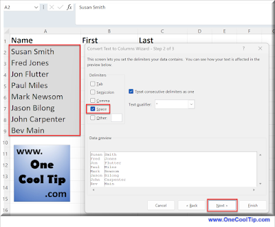
    • If you chose Delimited, you’ll need to specify the delimiters (comma, space, tab, etc.). 
    • If you chose Fixed Width, you’ll set where the column breaks should be.

Microsoft Excel Text to Columns Wizard
fig. 1 - Microsoft Excel Text to Columns Wizard

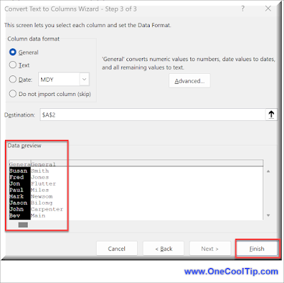
  • Next and Finish: You’ll get a preview of your data. 
Microsoft Excel Text to Columns - Preview
fig. 2 - Microsoft Excel Text to Columns - Preview
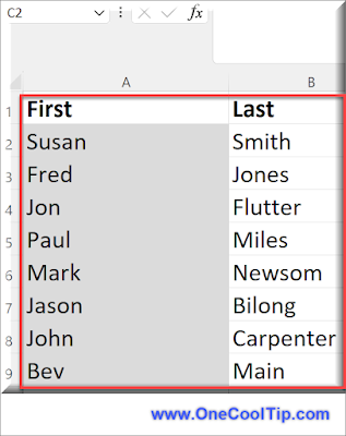
  • If everything looks good, click Finish.
Microsoft Excel Text to Columns - Final

fig. 3 - Microsoft Excel Text to Columns - Final

That's it!

Excel’s Text-to-Columns feature is a powerful tool that can save you time and frustration when dealing with complex data sets. 


Enjoy!

Please LIKE and SHARE OneCoolTip.com!


READ MORE

OneCoolTip.com
Cool Tech Tips for a Cooler Life

#Microsot @Microsoft #ExcelTips #DataAnalysis #TextToColumns #MicrosoftExcel #ProductivityHacks #BackToWorkMonday #TechTips #OneCoolTip @OneCoolTip #YouTube 

Monday, October 9, 2023

How to View Hyperlink Links in Microsoft Word

Microsoft Word
Have you ever found yourself lost in a sea of hyperlinks while working on a Microsoft Word document? 

Ever wished there was a way to view and manage all those hyperlinks effortlessly?

Here's a Cool Microsoft Word Tip.  Alt + F9

Hyperlinks are a powerful tool for creating interactive documents, but they can also be a bit mysterious.

Alt + F9 toggles the  hyperlink view in Microsoft Word. 

This allows you to see the underlying field code for a hyperlink, which can be helpful for troubleshooting or customizing hyperlinks.

Here's how to do it.
  • Open the Microsoft Word document containing the hyperlinks you want to view.

Microsoft Word Hyperlink
fig. 1 - Microsoft Word Hyperlink
  • Press Alt + F9.
  • This toggles the hyperlink view. 
Microsoft Word Hyperlink Alt + F9
fig. 2 - Microsoft Word Hyperlink Alt + F9
  • All hyperlinks in your document will be displayed in their raw format, showing the underlying URL instead of the display text.
  • To toggle back to regular view, press Alt + F9 again.

If you're editing a hyperlink, you can make changes to the field code directly in hyperlink view.

Enjoy!


Please LIKE and SHARE OneCoolTip.com!

READ MORE

OneCoolTip.com
Cool Tech Tips for a Cooler Life


#Microsoft @Microsoft #Word #MicrosoftWord #HyperlinkView #AltF9 #ALT+F9 #Technology #Productivity #TechTips #OneCoolTip @OneCoolTip #YouTube

Monday, October 2, 2023

How to Transpose Data in Microsoft Excel

Microsoft Excel
Have you ever found yourself in a situation where you needed to switch rows to columns or vice versa in your data? 

Ever wished for a magic wand that could instantly reorient your data to suit your needs? 


Here's a Cool Tip.  Microsoft Excel’s Transpose feature.

The Transpose feature in Excel is a tool that allows you to rotate your data by converting columns into rows, and rows into columns. 

This can be particularly useful when you want to restructure your data to make it easier to read or analyze. 

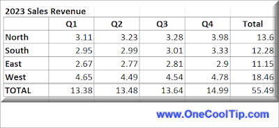
For example, if you have a dataset where the variables are in rows and observations are in columns, you might want to transpose the data so that each variable has its own column. 

This can make it easier to carry out further analysis, such as calculating descriptive statistics for each variable. 

The Transpose feature in Excel makes this process quick and easy, saving you the time and effort of manually rearranging your data.

Here's how to do it.
  • Select the data you want to transpose. 
  • Click and drag your mouse across the cells to select them.


fig. 1 - Selected Data to Copy in Excel

  • Copy the selected data
  •  You can do this by right-clicking on the selected cells and choosing ‘Copy’, or simply by pressing Ctrl+C  keys (Cmd+C for Mac users).
  • Click on the cell where you want your transposed data to begin. 
    • This will be the top-left cell of your transposed data.
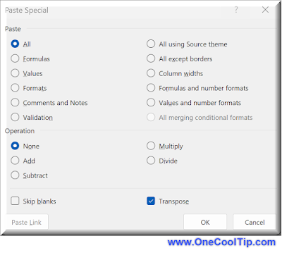
  • Right-click on the chosen cell and select ‘Paste Special’. 
    • A dialog box will appear.
  • In the ‘Paste Special’ dialog box, look for the ‘Transpose’ option and check it. 
  • Click ‘OK’.

Microsoft Excel Transpose Window
fig. 2 - Microsoft Excel Paste Special - Transpose Window

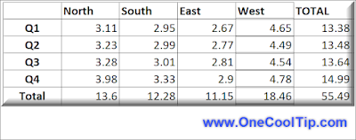
  • Your data has been transposed.

Transposed Data in Excel
fig. 3 - Transposed Data in Excel


Remember, if you have any formulas in your data, they will be adjusted to suit the new orientation. 

So, are you ready to take control of your data?

Enjoy!

Please LIKE and SHARE OneCoolTip.com!


READ MORE

OneCoolTip.com
Cool Tech Tips for a Cooler Life

#Microsoft #Excel @Microsoft #MicrosoftExcel #MicrosoftTranspose #DataManagement #ExcelTips #TechBlog #TechTips #OneCoolTip @OneCoolTip 

Monday, September 11, 2023

How to Master Formulas in Microsoft Word

Have you ever found yourself wishing you could perform calculations right within your Word document? 

Have you ever wondered how to make your tables in Word more dynamic and functional? 

Here's a Cool Tip:  Use the Formula feature in Microsoft Word.

That's right.

Formulas in Microsoft Word.

Microsoft Word offers a powerful feature that allows you to use formulas within tables, much like in Excel. 

Let's walk through  the process of using the formula function in Microsoft Word and explain the concept of positional arguments.


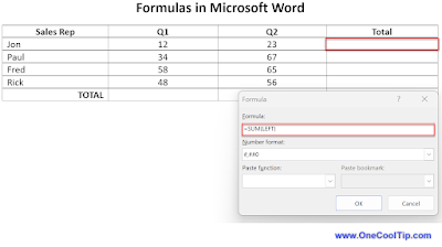
Formulas in Microsoft Word
fig. 1 - Formulas in Microsoft Word

Here's how to do it.
  • Insert a table into your Word document where you want to perform calculations.
  • Fill the cells with the data you want to calculate.
  • Click on the cell where you want the result of your calculation to appear. 
    • If the cell is not empty, delete its contents. 
  • Go to the Layout tab, in the Data group, and click on Formula.
  • Begin your formula with an equal sign, followed by your chosen function.
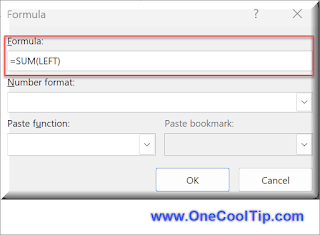
Word Formula
fig. 2 - Word Formula
  • Enter a function in the Formula field, such as SUM, AVERAGE, COUNT, MAX, MIN, PRODUCT.
    • Click on Paste function to select a function.
  • Use Positional Arguments: In the parentheses that follow the function, add positional arguments like LEFT, RIGHT, ABOVE, BELOW
    • These refer to the relative position of the cells that you want to include in your calculation.
Notes:

  • Update Formula Results
    • The result of a formula is calculated when it is inserted and when the document containing the formula opens. You can also manually update the result of one or more specific formulas by selecting them and pressing F9.
  • Understanding Positional Arguments
    • Positional arguments are used to refer to cell positions relative to the cell containing the formula. For example, if you want to sum numbers in a column above a specific cell, you would use the argument ABOVE in your SUM function.
With these steps, you can now perform calculations right within your Word document. 

No more switching back and forth between Word and Excel for simple calculations!

Enjoy!


Please LIKE and SHARE OneCoolTip.com!


READ MORE

OneCoolTip.com
Cool Tech Tips for a Cooler Life


#Microsoft #Word #MicrosoftWord #FormulasInWord #WordTips #Productivity #TechTips #OneCoolTip @Microsoft @OneCoolTip