Showing posts with label Microsoft Excel. Show all posts

Monday, October 16, 2023

Unleash the Power of Excel's Text-to-Columns Feature

Microsoft Excel
Ever found yourself staring at a jumbled mess of data in an Excel spreadsheet, wishing you could magically separate it into neat, individual columns? 

Have you ever wondered if there’s a simple way to transform a single column of data into multiple ones? 

Here's a Cool Tip.  Use Microsoft Excel’s Text-to-Columns feature.

Text to columns in Excel is a method that is used to separate a text into different columns based on some delimited or a fixed width.

Here's how to do it.
  • Click on the column or select the area that contains the data you want to separate.
  • Navigate to the Data tab on the Ribbon, 
  • Click on Text to Columns
  • A wizard will pop up.
  • Choose Your Data Type: 
    • You’ll be asked if your data is Delimited or Fixed Width
      • Delimited means your data is separated by characters such as commas or tabs. 
      • Fixed Width means the data is separated by a fixed number of spaces
    • Choose the option that fits your data.
  • Set Delimiters or Column Breaks: 
    • If you chose Delimited, you’ll need to specify the delimiters (comma, space, tab, etc.). 
    • If you chose Fixed Width, you’ll set where the column breaks should be.
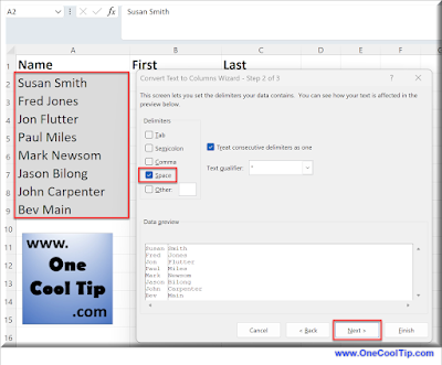
Microsoft Excel Text to Columns Wizard
fig. 1 - Microsoft Excel Text to Columns Wizard

  • Next and Finish: You’ll get a preview of your data. 
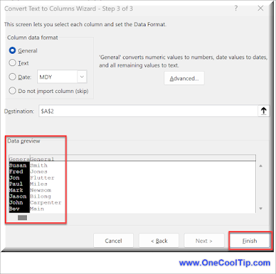
Microsoft Excel Text to Columns - Preview
fig. 2 - Microsoft Excel Text to Columns - Preview
  • If everything looks good, click Finish.
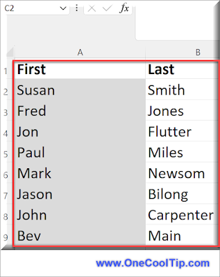
Microsoft Excel Text to Columns - Final

fig. 3 - Microsoft Excel Text to Columns - Final

That's it!

Excel’s Text-to-Columns feature is a powerful tool that can save you time and frustration when dealing with complex data sets. 


Enjoy!

Please LIKE and SHARE OneCoolTip.com!


READ MORE

OneCoolTip.com
Cool Tech Tips for a Cooler Life

#Microsot @Microsoft #ExcelTips #DataAnalysis #TextToColumns #MicrosoftExcel #ProductivityHacks #BackToWorkMonday #TechTips #OneCoolTip @OneCoolTip #YouTube 

Monday, October 2, 2023

How to Transpose Data in Microsoft Excel

Microsoft Excel
Have you ever found yourself in a situation where you needed to switch rows to columns or vice versa in your data? 

Ever wished for a magic wand that could instantly reorient your data to suit your needs? 


Here's a Cool Tip.  Microsoft Excel’s Transpose feature.

The Transpose feature in Excel is a tool that allows you to rotate your data by converting columns into rows, and rows into columns. 

This can be particularly useful when you want to restructure your data to make it easier to read or analyze. 

For example, if you have a dataset where the variables are in rows and observations are in columns, you might want to transpose the data so that each variable has its own column. 

This can make it easier to carry out further analysis, such as calculating descriptive statistics for each variable. 

The Transpose feature in Excel makes this process quick and easy, saving you the time and effort of manually rearranging your data.

Here's how to do it.
  • Select the data you want to transpose. 
  • Click and drag your mouse across the cells to select them.


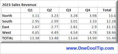
fig. 1 - Selected Data to Copy in Excel

  • Copy the selected data
  •  You can do this by right-clicking on the selected cells and choosing ‘Copy’, or simply by pressing Ctrl+C  keys (Cmd+C for Mac users).
  • Click on the cell where you want your transposed data to begin. 
    • This will be the top-left cell of your transposed data.
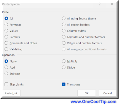
  • Right-click on the chosen cell and select ‘Paste Special’. 
    • A dialog box will appear.
  • In the ‘Paste Special’ dialog box, look for the ‘Transpose’ option and check it. 
  • Click ‘OK’.

Microsoft Excel Transpose Window
fig. 2 - Microsoft Excel Paste Special - Transpose Window

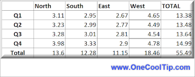
  • Your data has been transposed.

Transposed Data in Excel
fig. 3 - Transposed Data in Excel


Remember, if you have any formulas in your data, they will be adjusted to suit the new orientation. 

So, are you ready to take control of your data?

Enjoy!

Please LIKE and SHARE OneCoolTip.com!


READ MORE

OneCoolTip.com
Cool Tech Tips for a Cooler Life

#Microsoft #Excel @Microsoft #MicrosoftExcel #MicrosoftTranspose #DataManagement #ExcelTips #TechBlog #TechTips #OneCoolTip @OneCoolTip 

Wednesday, September 20, 2023

How to Set Tab Colors in Microsoft Excel

Microsoft Excel
Do you find yourself lost in a sea of identical Excel tabs? 

Have you ever wished for a way to visually distinguish your data sets? 

Here's a Cool Tip: Color-Code Your Excel Tabs,

Setting tab colors makes it easier to see your different tabs.


Here's how to do it.
  • Launch Microsoft Excel
  • Open the spreadsheet where you want to color the tabs.
  • Click on the tab you want to color. This will make it the active tab.
  • Right-click on the tab
  • Select Tab Color from the context menu. 
    • This will open a dialog box with color options.
  • Select your desired color from the palette. 
    • The tab will instantly change to reflect your choice.
  • Repeat steps for any other tabs you wish to color.

Set Tab Color in Microsoft Excel
fig. 1 - Set Tab Color in Microsoft Excel


That's it!

Enjoy!

Please LIKE and SHARE OneCoolTip.com!


READ MORE


OneCoolTip.com
Cool Tech Tips for a Cooler Life


#Microsoft @Microsot #Excel #Tabs #Color #MicrosoftExcel #DataOrganization #TechTips #ProductivityHacks #OneCoolTip @OneCoolTip

Saturday, September 16, 2023

Windows Super Secret Keyboard Shortcuts to Open Microsoft Applications

Microsoft Windows
Do you think you know Windows?

Do you know the super secret keyboard shortcuts to open Microsoft Applications?

There's even one to open the Microsoft-owned LinkedIn website.

Here's a Cool Tip:  Secret Microsoft Application Keyboard Shortcuts.

 
Here's how to do it.

  • Press and hold the Control + Shift + Alt + Windows + a letter from the list below for each application.
  • For example, L for LinkedIn.

Application

Windows Keyboard Shortcut

LinkedIn

CTRL + SHIFT + ALT + WIN + L

Word

CTRL + SHIFT + ALT + WIN + W

Excel

CTRL + SHIFT + ALT + WIN + X

PowerPoint

CTRL + SHIFT + ALT + WIN + P

Outlook

CTRL + SHIFT + ALT + WIN + O

Microsoft Teams

CTRL + SHIFT + ALT + WIN + T

OneDrive

CTRL + SHIFT + ALT + WIN + D

OneNote

CTRL + SHIFT + ALT + WIN + N


The keyboard shortcut to open LinkedIn on Windows is CTRL + SHIFT + ALT + WIN + L. 

This shortcut opens LinkedIn in your default browser. 

You can also use this shortcut to open other Office apps, including Word, Excel, PowerPoint, Outlook, Microsoft Teams, OneDrive and OneNote.

That's it!

Enjoy!


Please LIKE and SHARE OneCoolTip.com!

READ MORE


OneCoolTip.com
Cool Tech Tips for a Cooler Life


#Microsoft #keyboardshortcut #LinkedIn #Word #Excel #PowerPoint #Outlook #MicrosoftTeams #OneDrive #OneNote #techtips #OneCoolTip #Microsoft 

Wednesday, September 6, 2023

How to Insert a Picture in a Cell in Microsoft Excel

Microsoft Excel
Have you ever wanted to insert a picture into a cell in Microsoft Excel, but didn’t know how? 

Do you want to make your spreadsheets more visually appealing and engaging? 

Is this even possible?

Here's a Cool Tip:  Use the New Insert Picture Inside Cell feature.

That's right.

You can now insert pictures inside an Excel cell and not just on top of it.

Previously, you could only insert a picture on top of cells.

This new feature is now available in the latest version of Microsoft Excel in Microsoft65.

Here's how to do it:
  • Open the worksheet where you want to insert the picture.
  • Select the cell where you want to insert the picture.
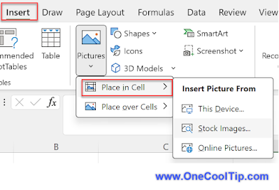
  • Click on the Insert tab in the ribbon at the top of the screen.
  • Click on the Pictures button in the Illustrations group.
  • Select Place in Cell.
  • Select where to Insert Picture From

Insert Picture in Cell in Microsoft Excel

fig. 1 - Insert Picture In Cell in Microsoft Excel
  • Navigate to the location of the picture and select it.
  • Click on the Insert button to insert the picture into the selected cell.

Picture Inside Cell in Excel

fig. 2 - Picture Inside Cell in Microsoft Excel

That's it!

Enjoy!


Please LIKE and SHARE OneCoolTip.com!


READ MORE

OneCoolTip.com
Cool Tech Tips for a Cooler Life!


Microsoft #Excel #MicrosoftExcel #ExcelTips #Spreadsheet #DataVisualization #TechTips #OneCoolTip @OneCoolTip @Microsoft #YouTube

Monday, August 28, 2023

Summing It Up: The Many Ways to Total in Microsoft Excel

Microsoft Excel
Have you ever found yourself needing to add up a long list of numbers? 

Whether you’re balancing your checkbook or calculating the total cost of a project, summing a series of numbers is a common task. 

But did you know that there are several ways to accomplish this? 

Here's a Cool Tip:  Use the Excel keyboard shortcut.

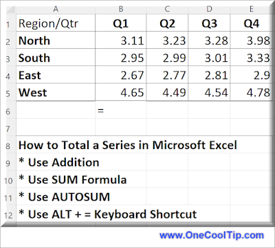
To total, or sum, a series of numbers in Excel, you can use several methods:

Use Addition:
  • This is a very simple method to add the value of several cells containing numbers together. 
  • Use the Formula: =A1 + A2 + A3 + A4  where A1, A2, A3 and A4 are the cells containing the numbers you want to total.
  • This works for a few cells but is unwieldly for a large set of numbers.

Use the SUM function:  
  • The SUM function is a built-in function in Excel that allows you to easily add up a range of cells. 
  • To use the SUM function, simply enter the formula =SUM(A1:A4) where A1:A4 is the range of cells containing the numbers you want to total.

Use AutoSum: 
  • AutoSum is a tool in Excel that automatically selects a column or row of numbers and calculates their sum. 
  • To use AutoSum, select the cell where you want to display the sum, then click on the AutoSum button in the toolbar on your screen.

Microsoft Excel Total Series
fig. 1 - Microsoft Excel Total Series


Super Cool Tip:

Use the Excel Keyboard Shortcut ALT + = to sum a series of numbers in a column or a row.

Enjoy!


Please LIKE and SHARE OneCoolTip.com!


READ MORE

OneCoolTip.com
Cool Tech Tips for a Cooler Life!

#Microsoft #Excel #MicrosoftExcel #SUM #TechTips #OneCoolTip @Microsoft @MicrosoftExcel @OneCoolTip 

Tuesday, August 22, 2023

How to Create a Series in Microsoft Excel: A Step-by-Step Guide

Microsoft Excel
Are you tired of manually entering data into your Excel spreadsheets? 

Do you want to save time and effort by automating the process of creating a series of numbers, days of the month, or days of the week? 

Here's a Cool Tip:  Let Excel create the series for you.

Creating a series in Excel is a simple and straightforward process. 

Here's how to do it:
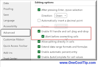
  • Ensure Excel’s AutoFill Options is turned on by going to File > Options > Advanced and checking the box next to Enable fill handle and cell drag-and-drop

Microsoft Excel Fill Handle Setting
fig. 1 - Excel Fill Handle Setting
  • Select the cell where you want to start your series.
  • Type the first few value of your series.
  • Select the fill handle at the bottom right corner of the selected cell.
  • Drag the fill handle in the direction you want to extend your series.
  • Release the mouse button to create your series.
For example, if you want to create a series of numbers from 1 to 10, you would type 1 into the first cell and 2 into the second cell, select the fill handle, and drag it down until you reach 10.  

Microsoft Excel Series
fig. 2 - Microsoft Excel Series

Excel will automatically fill in the rest of the numbers for you.

You can also create a series of dates or days of the week by following the same steps. 

Simply type the first month or day into the first cell, select the fill handle, and drag it down or across to create your series.

Save time and effort when entering data into your spreadsheets!

Enjoy!


Please LIKE and SHARE OneCoolTip.com!


READ MORE

OneCoolTip.com
Cool Tech Tips for a Cooler Life!

#Microsoft #Excel @Microsoft #MicrosoftExcel #ExcelSeries #ExcelTips #ExcelTutorial #TechTips #OneCoolTip @OneCoolTip 

Monday, August 14, 2023

Say Goodbye to Duplicates: How to Remove Duplicate Data in Excel

Microsoft Excel
Are you tired of dealing with duplicate data in your Excel spreadsheets? 

Do you want to learn how to quickly and easily remove duplicates from your data? 

Here's a Cool Tip:  Remove Duplicates in Excel

Here's how to do it.
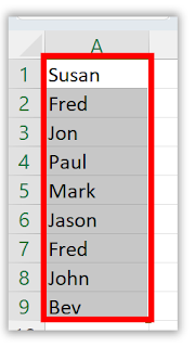
  • Select the range of cells that contains the duplicate values you want to remove 

Select Columns of Data
fig. 1 - Select Columns of Data

  • Click the Data tab in the Excel ribbon
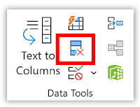
  • Click the Remove Duplicates button in the Data Tools group 
Excel Remove Duplicates
fig. 2 - Remove Duplicates

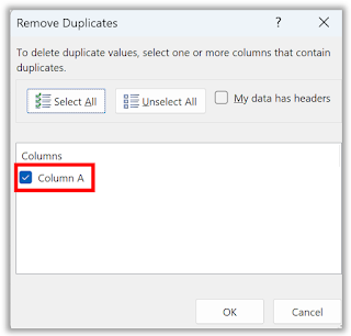
  • In the Remove Duplicates dialog box, check or uncheck the columns where you want to remove the duplicates 
Excel Select Columns to Remove Duplicates
fig. 3 - Select Columns to Remove Duplicates

  • Click OK.
Excel Remove Duplicates Alert
fig. 4 - Excel Remove Duplicates Alert

With these simple steps, you can quickly and easily remove duplicate data from your Excel spreadsheets. 

You can also turn on the Filter feature to help you find and remove duplicates more easily.


Enjoy!

Please Like and Share OneCoolTip.com!

READ MORE

OneCoolTip.com
Cool Tech Tips for a Cooler Life!


#Microsot #Excel #ExcelTips #DataCleaning #NoMoreDuplicates #TechTips #OneCoolTip @OneCoolTip @Excel @Microsoft

Monday, July 31, 2023

How to Format Cells with Color with This Excel-lent Cool Tip!

Microsoft Excel
Are you tired of constantly clicking through menus to format your cells in Microsoft Excel? 

Do you want to save time and increase your productivity? 

Look no further! 

Here's a Cool Tip: Use keyboard shortcut ALT+H+H. 

This allows you to quickly format cells with background colors in Excel.

When you press these keys, the Fill Color menu will appear, allowing you to quickly change the background color of a cell.

To use this shortcut, 
  • Select the cell or range of cells that you want to format. 
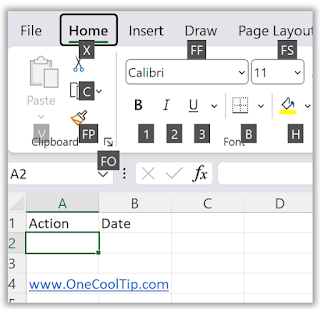
  • Press the ALT key
Microsoft Excel ALT Command
fig. 1 - Microsoft Excel ALT Command

  • Then press the H key twice
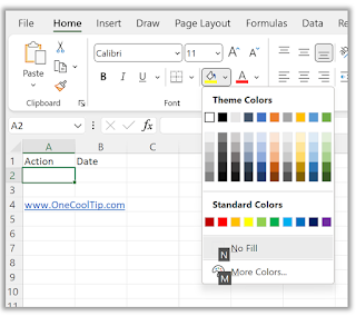
  • The Fill Color menu will appear.
Microsoft Excel Color Fill Menu
fig. 2 - Microsoft Excel Color Fill Menu
  • Use the arrow keys or your mouse to select the desired color.
That's it!

Using keyboard shortcuts can greatly improve your efficiency when working with Excel. 

Enjoy!

Check out how to use this Cool Tip on YouTube:

How to Do It - YouTube


Please Like and Share OneCoolTip.com!


READ MORE

OneCoolTip.com
Cool Tech Tips for a Cooler Life!

#Microsoft #MicrosoftExcel #ExcelTips #KeyboardShortcuts #Productivity @Microsoft #techtips #OneCoolTip 

Monday, July 17, 2023

Say Goodbye to Calibri - Hello Aptos!

Do you use Microsoft Office?

If so, there's a change coming with the default font.

Microsoft has announced that it is replacing its default font, Calibri. 

This change comes after 15 years of Calibri being the default font for Microsoft Office. 

The new default font is called Aptos.

But here's a Cool Tip:  You can already ready use it since it's currently called Bierstadt

Microsoft Default Font Aptos
fig.1 - Microsoft New Default Font Aptos and Previous Fonts


The decision to choose Aptos as the new default font was based on user feedback, with Aptos striking a balance between professionalism and relatability.

The new font will gradually become the default across all Microsoft 365 apps and services for all users over the coming months. 

However, Calibri will still be pre-pinned at the top of a new font menu alongside its predecessors, Times New Roman and Arial.

Please Like and Share OneCoolTip.com!


READ MORE

OneCoolTip.com
http://www.onecooltip.com
Cool Tech Tips for a Cooler Life!


#Microsoft #Aptos #NewFont #DefaultFont #MicrosoftOffice #Office #Microsot365 #Word #Excel #PowerPoint #Outlook #TechTip #OneCoolTip @Microsoft 


Source: Microsoft Design

Monday, July 3, 2023

How to Ensure Accurate Data Entry in Microsoft Excel

Microsoft Excel
Have you ever struggled with inaccurate date entries in your Excel spreadsheets? 

Do you want to ensure that the dates entered in your workbook fall within a specific range? 

Here's a Cool Tip: Use data validation to restrict date entries in Excel

Data validation is a powerful feature in Excel that allows you to control the type of data entered into a cell. 

With data validation, you can specify that a cell can only accept values that meet certain criteria, such as a date within a specific range.

Here's how to do it:
  • Select the cells where you want the data validation applied.
  • In the Ribbon, select Data > Data Validation.
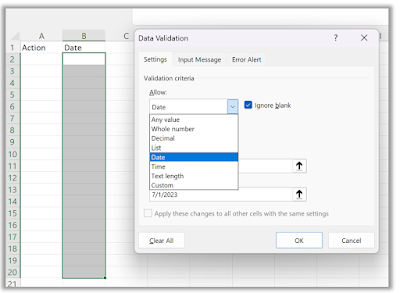
  • In the Settings tab, set the Validation criteria.
  • Set the Allow to Date
Microsoft Excel Data Validation
fig. 1 - Microsoft Excel Data Validation
  • Set the date range you want to apply.
  • Now, if a user tries to enter a date outside of the specified range, an error message will appear.
  • This helps ensure that the dates entered in your workbook are accurate and fall within the desired range.
You can choose many different data validations such as whole number, time, decimal or make your own Custom validation. 

You can also set the error message to display.

So use Data Validation the next time you are creating a spreadsheet for data entry.

Enjoy!

Please Like and Share OneCoolTip.com!

READ MORE

OneCoolTip.com
Cool Tech Tips for a Cooler Life!

#Microsoft #Excel #software #techtip #BacktoWorkMonday #MicrosoftExcel #DataValidation #Productivity #OneCoolTip @Microsoft